Author: Juan de Dwios Ortuzar and Luis G. Willumsend
Tags: #transportation #books #academic
👆 Short Summary (1 takeaway)
Comprehensive review of the historical and current state of practice for transportation modelling
🧐 Why I am reading this book?
To review the core concepts of transportation modelling in preparation for new job at Tesla
[[February 20th, 2021]] 5 month in, I have not really made use of this knowledge actively. There are some tangential thought experiments that brings some up but maybe 20% useful
The demand for transportation is derived, people don't travel (except sightseeing) for the sake of travel, it is often to satisfy a need (work, school, shopping)
A good transportation system widens the opportunities to satisfy these needs
Transport demand has strong dynamic elements, it peaks with direction, time, and space
This makes modelling demand interesting but also difficult
The supply for transportation is a service and not a good
Thus, you can't stock it and prepare it for high demand
Transportation systems are comprised of two things: fixed assets (infrastructure) and mobile units (vehicles)
These two things and a set of rules on how these two things coordinate makes up any transportation system
Investment in transportation infrastructure is lumpy and takes a long time to carry out
Also creates disruption to the existing service
Most importantly, infrastructure for transportation is largely political for most countries
Congestion occurs when the demand for the infrastructure approaches or reaches the capacity it can service
There is a perceived cost of congestion for all users due to the longer travel time
There is also an external cost added to all other users with each additional user
The role of transportation planning is to satisfy both short-term and long-term supply and demand
Development trap occurs when car-ownership increases, people can live and work irrespective of transit development which leads to urban sprawl - low-density development that is ineffectively served by public transit, which leads to further congestion.
Substantive rationality: people know their objective and evaluates the different choices to achieve their objective 2. This assumption is has problems with specifying the objective beyond cost-related measures and alienation of decision makers who do not accept this analytical style of thinking
Muddling through: people mix various high-level objectives, intermediate goals, immediate actions as an approach to make decisions
It is much better to be roughly right than precisely wrong - John Maynard Keynes
There are 4 main dimensions of model resolution
Space: from zones to addresses
Unit of analysis: from trips to household/person stratas to synthesized individuals
Behavioural responses: route choice actions, changes in time of travel, mode, destination, tour frequency, and even land use and economic activity impacts
Time: can be discrete or continuous. Discrete time can cover a full day (national models), time periods or smaller time intervals. Continuous time can allow for dynamic handling of traffic and behavioural responses
Main usage of models in practice is for conditional forecasting which is producing estimates for a dependent variables based on independent variables
Aggregate and disaggregate modelling
a key design decision based on the availability of data and the need for the model
Aggregate models were the norm up to 1970s, but they are criticized for inflexible, inaccurate and costly
Dissagregate models started to be popular during 1980s, but they require high statistical and economietric skills from the modeller
The main difference lies in the treatment of the description of behaviour, particularly during the model development process
Cross-section or time-series
Cross-section approach assumes that a measure of the response to incremental change may simply be found by computing the derivatives of a demand function with respect to the policy variables in question
this brings up two drawbacks, a given cross-sectional data set may correspond to a particular 'history' of changes and data collected at only one point in time will usually fail to discriminate between alternative model formulations
This led people to believe that where possible, longitudinal or time-series data should be used to construct more dependable forecasting models
Revealed and stated preferences
Observations on varies circumstances and reactions in transportation is often not available, and is was almost axiomatic that modelling transport demand should be based on revealed preference data
Stated preference techniques, borrowed from market research, were put forward as a way of experimenting with transport-related choices
Zone and network system -> Collection of planning and transportation data (base year and forecast) -> Trip generation -> Trip distribution -> Mode split -> Assignment
Expected value is the weighted average times probability
==Normal distribution has a mean of 0 and variance of 1==
==Central Limit Theorem states if we have n variables x that distribute with any distribution with finite variance, it can approach normal distribution after "standardizing" and if n is greater than or equal to 30==
Maximum likelihood is the most well-known and often used method of estimating parameters to deduce population characteristics from sample data
Good estimators are unbiased, or at least asymtotically unbiased
They are efficient, minimal variance
They are consistent
Hypothesis testing is based on taking a hypothesis and using to sample to verify that if null Hypothesis is true and we can accept the null Hypothesis or the null Hypothesis is false and we can reject the null Hypothesis
The Type I and II errors occur when we see the opposite
It is ideal to have low probability of both errors, but it is impossible to decrease the likelihood of one error without increasing the likelihood of the other error
The goal of modelling is forecasting, thus an important problem is to find which combination of model complexity and data accuracy best fits the required forecasting precision and study budget
Errors that affect this are:
Those that could cause even correct models to yield incorrect forecasts (errors in the prediction, transference and aggregation errors)
Those that actually cause incorrect models to be estimated (measurement, sampling and specification)
Measurement errors are inherent in the process of measuring the data, can be improved with better data-collecion process
Another common problem is the perception error inherent to the traveller when they report data
Sampling errors arise due to finite data sets, and to improve them requires squared effort
Specification errors are due to the misunderstanding or lack of understanding of the problem which can cause modellers to include irrelevant variables, omission of relevant variables, not allowing for taste variations on the part of the individuals, inappropriate model formulation
Transfer errors occurs when the model developed for a specific context is inappropriately applied in another (time and space), although the ones from temporal transfer might need to be accepted
Aggregation errors are the result of forecasting for a group of individuals when the modelling was estimated on individuals
The duality of model complexity and data accuracy is a constant struggle for modellers
Concentrate the improvement effort on those variables with a large error
Concentrate the effort on the most relevant variables
This chapter contains information to help design a travel demand survey of various kinds, which is not relevant for me right now
Current best practice suggests that the data set should have the following:
Consideration of stage-based trip data, relate specific modes to specific locations/times of day/trip lengths
Inclusion of all modes of travel
Measurements of highly disaggregated levels of trip purposes
Coverage of the broadest possible time period
Data from all members of the household
Information robust enough to be used even at a disaggregate level
Part of an integrated data collection system incorporating household interviews as well as origin-destination data from other sources such as cordon surveys
Data sources include:
Household surveys, used to generate data for trip generation, distribution and mode split
Intercept surveys: external cordons, used to catch people crossing the study border, and internal cordons
Traffic and person counts, for calibration and validation
Travel time surveys, for calibration and validation
Other related data
Land-use inventory which gives the modeller information on zone types, parking spaces
Infrastructure and services inventories which gives public and private transport networks, fares, frequencies, traffic signals
Information from special surveys on attitudes and elasticity of demands
Not enough data on alternative choices to give variability
Not enough information will be revealed to analyze secondary factors such as security, decor, and publicly displayed information on a user's decision
Lack of data for entirely new modes without good substitute
Contingent Valuation (CV), conjoint analysis (CA) and stated choices (SC) are three SP techniques with SC being the most common
CV deals solely with eliciting willingness-to-pay information for various policy or poduct options
4 types of CV questions are direct questioning, biding games, payment options and referendum choices
CA examines the preferences, and even WTP, not only for the entire policy as a whole, but also of the individual characteristics of the object(s) under study
CA surveys have heavy criticism, so it is not often used
SC is similar to CA insofar as a set of alternatives are presented, but instead of ranking them, the respondents are asked to choose their preferred alternative from among a subset of the total number of hypothetical alternatives constructed by the analyst
SC also typically presets a small subset of all available alternatives, changing this subset during the survey
Biggest issue is the how much faith can we put on individual actually doing what they state they would do
Early on, in 1970s only 50% of the people seem to actually do what they state and later on this improved
This could be because the data-collection method improved
Zoning system is used to aggregate the individual households and premises into manageable chunks for modelling purposes'
zone size must be such that the aggregation error caused by the assumptions that all activities are concentrated at the centroid is not too large
should be compatible with other administrative divisions, particularly census
should be homogeneous as possible in their land use and/or population
zone boundaries must be compatible with cordons and screen-lines
shape of the zones should allow for easy determination of their centroid connectors
zones do not have to be of equal size
Network is a key component of the supply side of modelling
normal practice is to model the network as a directed graph
links are characterized by several attributes such as length, speed, number of lanes and so on
one should include in the network at least one level below the links of interest
Most current assignment techniques assume that drivers seek to minimize a linear combination of time, distance, and tolls, or generalized cost of route choice
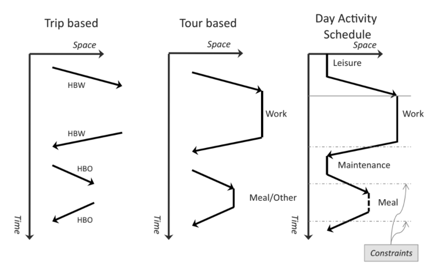
Sojourn is a short period of stay in a particular location, is usually associated with a purpose (work, study, shopping, leisure)
Activity is an endeavor or interest often associated with a purpose but not necessarily linked to a fixed location
It has been found in practice that a better understanding of travel and trip generation models can be obtained if journeys by different purposes are identified and modeled separately
travel to work
travel to school
shopping trips
social and recreational journeys
escort trips
other journeys
Mandatory (compulsory) trips are work and schools trips, while discretionary (optional) trips are the other types
Classification with respect to time of day is also useful, there are distinct traits for the AM/PM/Offpeak periods
Classification with person type or household type such as income level, car ownership, household size, family structure is also important
Trip production factors
Income, car ownership, family size, household structure, value of land, residential density, and accessibility
Accessibility have been studied for its affect on trip generation, but is rarely used in practice even though it can give valuable elasticity from changes in the transportation system
Trip attraction factors
roofed space for industrial, commercial, and other services, zonal employment, and accessibility
For Tesla, modelling trip attraction with supercharging stations could be interesting. Also, trip production should have a robust model for non-tesla behavior, so one can study the shift of tesla users and see elasticity on the tesla trip generation
Freight trip production and attraction factors
number of employees, number of sales, roofed area of firm, and total area of firm
Growth factor modelling is the simplest technique for trip generation
Future Trips = Growth Factor x Current Trips
Growth Factor = f(Future population, income, car ownership)/f(Current population, income, car ownership)
Mainly used to predict future number of external trips because this is a crude method and is prone to overestimate but requires little data
Moving beyond growth factor modelling, one can use linear regression to find the relationship between the number of trips produced or attracted by zone and average socioeconomic characteristics of the households in each zone
this can only be successful if the inter-zonal variations adequately reflect the real reasons behind trip variability. A major problem is that the main variations in person trip data occur at the intra-zonal level
it is common to have a large intercept value from estimation, which means the equation may be rejected. One would expect the estimated regression line to pass through the origin
null zones needs to be excluded from analysis
zone totals vs zone means. The use of aggregate variables implies that the magnitude of the error actually depend on zone size, this heteroskedasticity has indeed been found in practice. Need to apply multipliers to reduce heteroskedasticity.
In the early 1970s, it was believed that the most appropriate analysis unit was the household
little practical success
Linear regression model assumes that each independent variable exerts a linear influence on the dependent variable
There are two methods to include non-linearity behavior
transform the variables in order to linearise their effect (log, ln, exp)
use dummy variables to discretize continuous variables into separate variables
Because trip generation models are often estimated on better variables and uses better data, to ensure generation totals match production totals it is common to scale the generation side to match the production side
A popular method in the UK, estimating the response (e.g. the number of trip production per household for a given purpose) as a function of household attributes)
The art of the method lies in choosing the categories such that the standard deviations of the frequency distributions are minimized
The advantages are
cross-classification groupings are independent of the zone system of the study area
no prior assumptions about the shape of the relationship are required
relationships can differ in form from class to class
The disadvantages are
model does not permit extrapolation beyond its calibration strata, although the lowest or highest class may be open ended
no statistical goodness-of-fit measures for the model
unduly large samples are required, accepted wisdom suggests that at least 50 observations per cell are required to estimate the mean reliably
there is no effective way to choose among variables for classification
if it is required to increase the number of stratifying variables, it might be necessary to increase the sample enormously
Read more in detail to see improvements for this basic model to have some statistical attributes extracted
The person-category approach is an alternative to the household-based model which offers some advantages
Biggest limitation is the difficulty of introducing household interaction effects and household money costs and money budgets into a person-based model
Classic specification of the four-stage model does not include trip generation in the iterative procedure, this means that network changes does not affect the number of trips generated
To solve this, modellers have attempted to incorporate a measure of accessbility into trip generation equations
replace O=f(H) by O=f(H, A) where H is household characteristics and A is a measure of accessibility by person type
accessibility measures take the general form A = sum(f(E, C)) where E is a measure of attraction of a zone, and C is the generalized cost of travel, a typical analytical form is: A = sum(E^alpha * exp(-beta * E))
But this has been unsuccessful in practice, insignificant or the wrong sign
Daly (1997) used the Logit form to predict the total number of trips by calculating the probability that each individual would choose to make a trip. Total travel volume can then be obtained by multiplying the number of individual of each type by their probabilities of making a trip
The preferred form of accessibility at the destination (or mode) choice model is the logsum
The stop-go trip generation model forms a hierarchical relationship for the individual to determine whether it will continue its tour at each stop or return home
This may be a key formulation to use for tesla in order to test how the availability of supercharging stations will change a user's journey length
4.6 Forecasting Variables in Trip Generation Analysis
It has become a topic of interest for the modelling group to be able to capture social circumstances in which individuals live through behavioral sceince
One way to achieve this is to develop a set of household types that effectively captures these distinctions and then add this measure to the equations predicting household behavior
consistent with the idea that travel is a derived demand and that travel behavior is part of a larger allocation of time and money to activities in separate locations
important stages in households for travel behavior might be
appearance of pre-school children
time when youngest child reaches school age
time when a youth leaves home
time when all the children left home but the couple has not yet retired
time when all members of a household have reached retirement age
Old trend of aging population which may result in less travel might not hold in the future with the advent of autonomous vehicle
Huge opportunity to study how autonomous vehicle technology change travel behavior, if this increases the number of discretionary trip making?
4.7 Stability and Updating of Trip Generation Parameters
A key and often implicit assumption of using cross-sectional data is that the model parameters will remain constant between the base and design years
it is found in several studies that this cannot be rejected when trips by all modes are considered together
other analyses have reported different results, which has the following implications
if there is non-zero elasticity of car trip rates to fuel prices, the usual assumption of constant trip rates in a period of rapidly increasing petrol prices could lead to serious over-provision of highway facilities
trip rates of electric vehicle and gasoline vehicle is different depending on the external prices of electricity and oil
Then, it is clear that any variables with longitudinal effects on trip rates requires careful consideration as it has fundamental importance
but this requires data where only cross-sectional data is available
Geographical stability (transferrability) is another important attribute of a robust travel demand model
it would suggest the existence of certain repeatable regularities in travel behavior which can be modeled
it would indicate a higher probability that temporal stability also exists
it may allow reducing substaintially the need for costly full-scale transportation surveys on different areas
It is equally clear that not all travel characteristics can be transferable (i.e. work trip duration), but trip rates should not be seen as unrealistic
Bayesian techniques can be used to update the parameters of an estimated model from one area to be applied to another area
requires a small sample of data in the application area
considers a prior distribution (estimated area) and new information to create a posterior distribution corresponding to eh application area
There are two ways of representing the pattern of travel
a trip matrix which represents the origin and destination of the trips
a PnA matrix which represents the production and attraction of the trips
Trip distribution is often seen as an aggregate problem with an aggregate model for its solution, however, the choice of destination can also be treated as a discrete choice (disaggregate) problem and treated with models at the level of the individual
Discrete choice model might be important for modelling existing Tesla users, since they may have strong considerations for proximity to charging station?
A generalized cost is often computed between all the O-D pairs
including travel time, wait time, walking time, fare, terminal cost, modal penalty
First used by Casey (1955) to model shopping trips between towns in a region
The popular version of this function is now a combined function of a negative exponential and power functions
The generalized function of travel cost looks like this:
f(cij)=cijα∗exp(−β∗cij)
Tij=Ai∗Oi∗Bj∗Dj∗f(cij)
A more general version accepts empirical values and depend only on the generalized cost of travel in the form of TLFD but instead of coming up with a single value for alpha and beta, there are as many parameters as there are bins
Key assumption made by this method is that the same shape or TLFD will be maintained in the future
Given a system with a large number of distinct elements, to describe such a system one would need a complete specification of its micro states. However, it is practical to work in meso-state, which can be arrived at many different micro states. Then there is a even higher level of aggregation, macro state, which is where one makes reliable observations about the system
The basis of this method is to accept that all micro states consistent with our information about macro states are equally likely to occur
this is done by expressing our information as equality constraints in a mathematical program
the most probable meso state is that one that can be generated the most often, so if we have a number of micro states WTij and macro state T_ij one can optimize the following
W{Tij}=sum(Tij!)T!
Taking log, then approximating and taking the derivative one gets:
log(W′)=−∑(Tijlog(Tij)−Tij)
Thus, by maximizing log(W') enables us to generate models to estimate the most likely meso states
This formulation with the appropriate constraints can be used to derive the Furness model or gravity model
An extension of the gravity model is to account for not just the deterrent effect of distance but also for the fact that the further away one is willing to travel the greater the number of opportunities to satisfy your needs
Fang and Tsao (1995) suggested a model called self-deterrent gravitymodel with quadratic costs:
exp(−β×Cij×−λ×Tij×Cij)
Another model is the intervening opportunities model, which says trip making is not explicitly related to distance but to the relative accessibility of opportunities for satisfying the objective of the trip
consider first a zone of origin i and rank all possible destinations in order of increasing distance from i
then look at one O-D pair where j is the mth destination in order of distance, there are m−1 alternative destinations actually closer to i
a trip maker would certainly consider those destinations as possible locations to satisfy the need given rise to the journey, which are the intervening opportunities influencing a destination choice
let α be the probability of a trip maker being satisied with a single opportunity, then the probabiliy of being attracted by a zone with D opportunities is αD
consider probability qim of not being satisfied by any of the opportunities offered by the mth zones, which is not being satisfied with first, second, or mth
qim=qim−1×(1−αDim)
q(x)=Ai×exp(−αx) where x is the cumulative attractions of the intervening opportunities
This formulation starts from a different first principles which is interesting
Not often used in practice because the theory behind it is less well known, can be difficult to handle when implemented, the advantages over gravity is not overwhelming, no suitable software
It can be treated as an aggregate problem similar to trip distribution, and we can observe how far we can get with similar tools
Examine direct demand models - a method to estimate generation, distribution and modal split simultaneously
Examine the need for consistency between parameters and structure of distribution and mode choice models
Often disregarded by practitioners at their peril
The issue of mode choice is arguably the most important element in transport planning and policy making - thus it is important to develop and use models which are sensitive to those attributes of travel that influence individual choices of mode
Reliability of travel times and regularity of service
Comfort and convience
Safety, protection, security
The demand of the driving task
Opportunities to undertake other activities during travel
A good mode choice model would be based at least on simple tours and should include factors such as if one takes a car for the first leg then it is likely for one to use the car on the subsequent legs
Integrates the trip characteristics because it is applied post-distribution but can be difficult to include user characteristics because the info may be lost in the trip matrix
Initially, empirical relationships with in-vehicle travel time was used to estimate what proportion of travellers would be diverted to use a longer but faster bypass route
S-curve
Another approach is to use a version of Kirchhoff formulation in electricity
The proportion of trip makers between i and j that chooses mode k as function of the respective generalized cost Cij is given by: Pijk=∑(Cijk)−n(Cijk)−n
Where n is a parameter to be calibrated or transformed from another location or time
This is not too dissimilar from the Logic equation
Entropy-maximizing approach can be used to generate models of distribution and mode choice simultaneously - which leads to the Logit form
Logit form
Pij1=∑exp(−βCijk)exp(−βCij1)
The parameter β plays two roles: it acts as the parameter controlling dispersion (trip distribution) and also in the choice between destinations at different distances (mode choice) from the origin
So a more practical joint distribution/modal-split modal has the form (Wilson 1974) which splits out β into two separate parameters
Where Kijn is the composite cost of travelling between i and j asp received by person type n
Williams (1977) showed that the only correct specification of K is
Kijn=λn−1log(∑(exp(−λnCijk)))
βn≤λn
The last equality is vital to ensure that the structure G/D/MS/A can be used, otherwise if β>λthen the structure G/MS/D/A could be the correct one
==For many applications these aggregate models remain valid and in use. However, for a more refined handling of personal characteristics and preferences we now have disaggregate models which respond better to the key elements in mode choice==
For a multi-modal scenario, the N-way structure is popular in disaggregate modelling work
but it assumes all alternatives have equal weight which can lead to problems if alternatives are correlated
[[blue-bus-red-bus]]
Another structure is the added-mode structure, which was popular in the late 1960s and early 1970s
But this has shown to give different results depending on which mode is taken as the added one
Also it has been shown that the form with good base year performance does not translate in forecasts
The standard practice in the 1960s and early 1970s was the nested structure where alternatives with common elements are grouped together
Shortcoming of this was the composite cost for the “public-transport” mode were normally taken as the minimum of costs of the bus and rail modes for each zone pair and that the secondary split was achieved through a minimum-cost “all-or-nothing” assignment
This implies an infinite value for the dispersion parameter of the sub-modal split function
Applying this form to [[blue-bus-red-bus]]
Calibrating a binary logit model with known proportions of choosing each mode and the cost of travel for all OD pairs across both modes is done with linear regression with the LHS of the following equation as dependent variable and the cost difference as the independent variable
log[(1−P1)P1]=λ(C2−C1)+λδ
Where λ is the dispersion parameter and δ is the modal penalty (assumed associated with the second mode)
Calibrating a hierarchical modal-split model involves recursion using maximum likelihood estimation (as opposed to least square estimates). Data is grouped into suitable cost-bins
First calibrate the sub-modal split using the technique above
Then, segment trips that have a choice in modes into bins
Calculate the weighted cost of each bin
The probability of choosing a mode for each bin can be represented as:
Pk=[1+exp(−Yk)]1
Yk is the representative cost of the bin
The logarithm of the likelihood function is:
L=constant+∑[(nk−rk)log(1−Pk)+rklog(Pk)]
nk is the observed number of trips in the cost-difference interval
rk is the observed number of trips by the first mode in the interval
Then by taking the partial first and second derivatives w.r.t various parameters, a search algorithm can find the maximum
Alternative to sub-models, this approach is to create one single model that consolidates generation, distribution and mode choice
Direct Demand Models use a single estimated equation to relate travel demand directly to mode, journey and person attributes
Quasi-Direct Models employ a form of separation between mode split and total OD travel demand
Direct Demand Models
Earliest forms use multiplication, there are different versions with different mathematical forms
SARC (Kraft 1968) model estimates demand as a multiplicative function of activity and socioeconomic variables for each zone pair and LOS attributes of the modes serving them
Rewritten (Manheim 1979) to a clean form of:
Tijk=θYikZjk∏m(Lijm)
Yik is a composite term for population and income at the origin
Zjk is a composite term for population and income at the destination
Lijm is a composite term for travel time and cost between OD and mode
Very attractive in principle, but the large number of parameters needed to estimate can be hard to capture correctly
==Commonly used in intra-urban studies where the zones are large, or places where the ere are unique OD patterns that can be captured better with direct demand models rather than gravity models==
Quasi-Direct Models
A combined frequency-mode-destination choice model where the structure is of Nested Logit form
The distribution-models split model is coupled with the choice of frequency (Trip Generation) via a composite accessibility variable
Discrete choice model postulate that: the probability of individuals choosing a particular option is a function of their socioeconomic characteristics and the relative attractiveness of the option
Utility is used to represent attractivness
Alternatives present utility to the user
There are observable utility and random utility
Observable utility is often represented by linear combination of variables with coefficients representing their relative effects
The intercept, or alternative specific constant represents the net influence of all unobserved utility such as comfort and convience
To predict, the utility of an alternative is transformed into a probability value
Logit formulation
Probit formulation
These models can’t be calibrated using standard curve-fitting techniques because their dependent variable is an un-observed probability and the observations are the individual choices
Random utility theory (Domencich and McFadden 1975)
Individuals act rationally and possess perfect information
There is a set of alternatives and a set of characteristics for these alternatives and the individuals
Each alternative has associated a net utility for the individual. Since the modeller does not have perfect information, the net utility Ujq is comprised of systematic utility Vjq and random utility ϵjq
The population is required to share the same set of alternatives and face the same constraints
The individual selects the maximum-utility alternative
Proposed by Domencich and McFadden in 1975, this is the simplest and most popular practical discrete choice model
The random residual is assumed to have a Extreme Value Type I distribution (Gumbel or Weibull)
The choice probability formulation is
Piq=∑(exp(βViq))exp(βViq)
There is an important issue called theoretical identification which is revisited in this chapter
==Discrete choice models require to set certain parameters to a given value in order to estimate the model uniquely==
An important property of this model is the satisfaction of the axiom of independence of irrelevant alternatives (IIA)
Where any two alternatives have a non-zero probability of being chosen, the ratio of one probability over the other is unaffected by the presence or absence of any additional alternative in the choice set
This is advantages when using it for a new alternative problem
Disadvantages when used with correlated alternatives 7.4 The Nested Logit Model (NL)
If there are too many alternatives, it can be shown that unbiased parameters are obtained if the model is estimated with a random sample of the available choice set for each individual
Direct and cross elasticities can be easily computed
In more complex situations, the MNL might be inadequate
When alternatives are not independent
When the variances of the error terms are not equal
Heteroskedasticity between observations because some user have GPS to measure time more accurately or between alternatives because wait time is more accurate for rail compared to bus
There are flexible models like the probit model, (see 7.5 The Multinomial Probit Model) anzd the mixed logit model (see 7.6 The Mixed Logit Model)
These present other challenges such as difficult to solve
Formally presented by Williams in 1977 and Daly and Zachary in 1978 independently from each other
U(i,j)=Uj+Ui/j
Where i denotes alternatives at a lower level nest and j the alternative at the upper level
U(i,j)=V(i,j)+ϵ(i,j)
Where like before, V(i,j)=V(j)+V(i/j) is the representative utility and ϵ(i,j)=ϵ(j)+ϵ(i/j) is the stochastic utility
Williams’ definition of the stochastic error terms may be synthesized as follows
The errors ϵ(j),ϵ(i/j) are independent for all (i,j)
The errors ϵ(i/j) are identically and independently distributed (IID) EV1 8th scale parameter λ
The errors ϵ(j) are distributed with variance σj2 and such that the sum of Uj and the maximum of Ui/j is distributed EV1 with scale parameter β
Such distribution may not exist
The structural condition of this model is still β≤λ
McFadden in 1981 generated the NL model as one particular case of the Generalized Extreme Value (GEV) discrete choice family (see 7.7 Other Choice Models and Paradigms)
Limitations of NL
This is not a random coefficients model, which means it can’t cope with taste variations among individuals without explicit market segmentation
It can’t treat heteroskedastic options, as the error variances of each alternative are assumed to be the same
It can only handle as many interdependencies among options as nests have been specified
If can’t handle cross-correlation effects between alternatives in different nests
The search for the best NL structure requires a priori knowledge
The stochastic utility errors are distributed multivariate Normal with mean zero and an arbitrary covariance matrix
==This mean the model can’t be written in simple closed form like the MNL (except in a binary case)==
To solve this, we need simulations
Binary Probit Model
U1(θ,Z)=V1(θ,Z)+ϵ1(θ,Z)
U2(θ,Z)=V2(θ,Z)+ϵ2(θ,Z)
P1(θ,Z)=Φ[(V1−V2)/σϵ]
Although Φ[x] is the cumulative standard Normal distribution which has tabulated values, the equation is not directly estimable
There is also an identifiability problem and one would need to normalize before obtaining an estimate of the model parameters
An important problem of fixed-coefficient random utility models (MNL and NL) is their inability to treat the problem of random taste variations among individuals without explicit market segmentation
MNP handles this problem with its error distribution form
A restriction of NL model is for modes like Park & Ride, it is correlated to both drive and rail
To tackle this, various types of GEV models have been formulated with overlapping nests
Cross-Nested Logit model
Cross-Correlated Logit model
Paired Combination Logit model
There have been criticism over linear-in-the-parameters form because they are associated with a compensatory decision-making process, a change in one or more of the attributes may be compensated by changes in the other
Choice by elimination
Satisficing behaviour
8.0 Specification and Estimation of Discrete Choice Models
How to fully specify a discrete or disaggregate model (DM)
Selecting the structure of the model
The explanatory variables to consider
The form in which they enter the utility function
Identification of the individual’s choice set
How to estimate such a model once properly specified
With readily available software?
A common issue is although we may be able to successfully estimate the parameters of widely different models with a given data set, these (and their elasticities) will tend to be different and we often lack the means to discriminate between them
First thing for modeller to decide is - which alternatives are available to each individual in the sample
Without asking the respondent what the available set of options are there, there is no good way of limiting the number of options
Take into account only subsets of the options which are effectively chosen in the sample
Brute force method of assuming everybody has all alternatives available
The decision maker may also only decide from a limited set of choices from the ones assumed by the modeller because of lack of knowledge (i.e. didn’t know there is a bus)
Use heuristic or deterministic choice-set generation rules which permit the exclusion of certain alternatives (i.e. bus is not available to someone if the nearest stop is x meters away)
Collection of choice-set information directly from sample, asking the respondents about their perception of available options
Use random choice sets from a two-stage process: first a choice-set generation process which a probability function picks from all possible choices, and secondly a conditional on the specific choice set, a probability of choice for each alternative is defined
Sufficiently large values of t, typically greater than 1.96 for 95% confidence level, can reject the null hypothesis and accept that this attribute has a significant effect
==Current practice recommends including a relevant (i.e. Policy type) variable with a correct sign even it if fails any significance test== because the estimated coefficient is the best approximation available for its real value and the lack of significance can be justified by the lack of data
A way to include socio-economic characteristic is to create interaction variables with the utility variables
essentially a partial segmentation procedure
Overall test of fit
Compare the model against a market share model
The ρ2 index
Defined as 1−l∗(0)l∗(Θ)
==Values around 0.4 are usually considered excellent fits==
There are two adjustments to this formulation to account for proportion of the choices and the number of parameters, known as correctedρ2 and adjustedρ2
Estimating from choice-based sample is difficult
Maximum likelihood estimators are impractical due to computational intractability
However, if the modeller knows the fraction of the decision-making population selecting each alternative, then a tractable method can be introduced. Weight the contribution of each observation to the log-likelihood by the ratio of the friction of the population selecting the option over sample selecting the option
MNP and ML (mixed logit) do not have a closed form, so their choice probabilities are characterized by a multiple integral that is not easy to solve efficiently
Solved with numerical integration if one wants the most accurate mouthed
There are two features of SP that will affect which analysis method to use
Each respondent may contriubte with more than one observation
Preference can be expressed in different forms
The preferred SP response is ranking because it is simpler and more reliable
There are four broad groups of techniques for analysis, they all seek to establish the weights attached to each attribute in an utility function estimated for each alternative, known as preference weights
Naive or graphical methods
Lease square fitting
Non-metric scaling
Logit and Probit analysis
Naive approach calculates the mean average rank and compares it with each alternative
Seldomly used in practice
Least square fitting is basically estimating an equation based on the response to predict the rating for the alternative
This can obtain a goodness of fit
Non-metric scaling is used with rank data
Monotonic Analysis of Variance or MONOANOVA has been used for this
==Travel demand models are required to forecast transportation changes and examine their sensitivity with respect to changes in the values of key variables==
Aggregate models have been overly used because of it offers a tool for the complete modelling process
Disaggregate models often lacks the data necessary to make aggregate forecasts
Econometric POV - the aggregation over unobservable factors results in a probabilistic decision model and the aggregation over the distribution of observable results in the conventional aggregate or macro relations
Given a set of data pertaining to individuals
One options to aggregate into groups and estimate macro-relations. Then using this macro-relation to produce aggregate forecasts
The alternative is to estimate micro-models. Then use these models to on individuals which is then aggregated to produce aggregate forecasts
The question is exactly how to aggregation the micro-relations
Generally, it is context dependent. It is clear for mode choice and short-term modelling that the use of highly disaggregate data is desirable
The immense majority of discrete choice model applications have failed to produce confidence intervals for the estimated probabilities
Despite having two methods of doing so: approximate the choice probabilities by a first order Taylor series expansion, solve a non-linear programming problem
While a disaggregate model allows us to estimate individual choice probabilities, we are normally more interested in the prediction of aggregate travel behaviour
If the choice model was linear, then the aggregation process would be trivial - replace the average of the explanatory variables for the group in the model - naive aggregation
If the choice model was non-linear then naive aggregation will produce a bias
So another method is to use a sample population and calculate the predicted market share of alternative A in population by multiplying the expansion factor by the predicted probability - sample enumeration
The problem with sample enumeration is that it maintains the assumption of the base year’s conditions, so it falls apart in long-term prediction
Another practical method called classification approach which approximates a finite number of relatively homogeneous classes
The accuracy of this method depends on the number of classes and their selection criteria
==It is unrealistic to expect an operational model in the social sciences to be perfectly specified, thus it is not useful to look for perfect model stability==
Model transference should be viewed as a practical approach to the problem of estimating a model for a study area with little resources or a small available sample
A transferred model cannot be expected to be perfectly applicable in a new context, updating procedures to modify their parameters are needed so that they represent behaviour in the application context more accurately
How to evaluate model transferability
By comparing model parameters and their performance in two context
Test model parameter for equality - if this holds then the null hypothesis that this difference is zero cannot be rejected at the 95% level
This method suffers from the scale problem
It can’t distinguish if the differences is real or a result of scaling
Disaggregate transferability measures - based on the ability of a transferred model to describe individual observed choices and rely on measures of [[log-likelihood]]
Two indices can be calculated from the difference in log-likelihood
Transferability test statistics (TTS) is the twice the difference in log-likelihood
The test is not symmetric
Transfer index (TI) is the degree to which the log-likelihood of the transferred model exceeds a null model (market share model) relative to the improvement provided by the model developed in the new context
Bounded at 1, negative values imply the transferred model is worse than the local reference model
How to update with disaggregate data?
Scale and bias parameters are introduced to fit using aggregate data in application
If viable, an alternative is to use purposely designed synthetic samples in an enumeration approach
The network system gives the model the supply side information in terms of frequency and capacity
It only provides a cost-model, how transport cost will change with different levels of demand
It doesn’t specify the optimal supply given then future demand
For , the model should have the ability to say given these subset of people who wish to travel using EV, how many stations are needed and at what locations such that they can complete their trips
Network equilibrium is reached when travellers from a fixed trip matrix all have optimized their route such there are no alternative routes that reduces their respective costs
System equilibrium is a higher level state when trip matrix has reached a state of stabilization as a result of the congestion from the network
==Note: this is different from the idea of network optimal and system optimal network assignments==
Speed-flow and cost-flow curves help define the relationship between the two variables
There are various forms proposed for different link classifications that gives specification to the general form of Ca=Ca(Va)
Smock (1962) for Detroit proposed t=t0exp(QsV) where t0 is the travel time under free flow and Qs is the stead-state capacity of the link
Overgaard (1967) generalized Smock’s equation to t=t0αβ(QV) where Q is the capacity of the link and α,β are parameters for calibration
Bureau of Public Roads (1964) proposed the most commonly used form oft=t0[1+α(QV)β]
Department of Transport in UK has a piece-wise function for urban, sub-urban and inter-urban roads
Akcelik (1991) proposed a curve that focuses on the junction and penalizes over capacity flows more with t=t0+(0.25T)[(x−1)+(x−1)2+QjT8JAx] where T is the flow modelling period (typically 1 hour), Qj is the capacity at the junction (there is a formula to find it), x is the QjV ratio, JA is the delay parameter
==It is recommended to consider both time and distance with a generalized cost of Ca=α(traveltime)a+β(linkdistance)a==
Obtain good aggregate network measures (total flows on links, total revenue by bus service)
Estimate zone-to-zone travel costs (times) for a given demand
Obtain reasonable link level flows and identify heavily congested links
Secondary objectives
Estimate routes used between each OD pair
Select link analysis
Obtain turning movements for the design of future junction
Basic assumption of assignment is that of a rational traveller
One that will choose a route with the least perceived individual cost
This perceived cost is a generalized cost between time, distance, monetary costs, congestion’s, queues, maneuvers, type of road, scenery, road works, etc
The most common approximation is to use time and monetary cost
There are factors that result in the trips in the same OD pair taking different routes
Differences in individual perception of what constitutes at the “best route”
Many of these methods use [[Monte Carlo simulation]] to represent the “randomness” in drivers’ perception
Burrell (1968) developed a popular method
For each link in a network, develop an objective cost and subjective cost. The subjective cost is a distribution with the objective cost as the mean
Burrell assumed a normal distribution, others hypothesized Normal distribution
The distribution of subjective costs are assumed to be independent
Drivers are assumed to choose route that minimizes their subjective cost over the entire route
A shortcoming of this is that the subjective costs are not independent, and lead to unrealistic switching between parallel routes connected by minor roads
Dial (1971) proposed a proportional stochastic approach that splits trips based on a logit formulation
There is ongoing research on how to integrate stochastic assignment methods closer with developments in discrete choice
Ignoring stochastic effects and just focus on congestion’s feedback on assignment, there is a different set of models
Wardrop (1952) proposed the following
Wardrop’s first principle
[[quotes]] "Under equilibrium conditions traffic arranges itself in congested networks in such a way that no individual trip maker can reduce their path costs by switching routes"
Also known as user optimal
Wardrop’s second principle
[[quotes]] "Under social equilibrium conditions traffic should be arranged in congested networks in such a way that the average (or total) travel cost is minimized"
Also known as system optimal
Braess’s Paradox
(not really a paradox)
Illustrates this two principles by demonstrating that under certain conditions adding capacity to a road network when drivers seek to minimize their own travel costs can actually increase the system cost
To solve these equilibriums there have been various methods proposed (exact and heuristic)
This presents the formal formulation of the assignment problem with mathematical programming
Frank-Wolfe algorithm (link flow)
A linear approximation method
Solves a line arises sub-problem to get a good descent direction and finds a new solution using linear search
Guarantees a reasonable convergence to Wardrop’s equilibrium
Jayakrishman’s Gradient Projection algorithm (route or path based)
Origin based assignment
A family of solution methods that define the solution variables in an intermediate way between links and routes
Stochastic equilibrium assignment combines the effects of stochasticity and user-optimal
Each user chooses the route with the minimum “perceived” travel cost
The difference between SUE and Wardrop’s user equilibrium is that each driver has a self-defined “travel cost” instead of a single global value for the class of drivers
The difficult part of implementing this is that it might not converge
Peak spreading phenomenon happens when congestion rises and travellers shift their departure time to avoid it
In a macro model, this can be modelled as a logit choice between travelling at different periods
Each period will have their respective advantages and disadvantages
However, overall there is not a lot of flexibility for mandatory trips to shift outside of the peak period
In a micro model, there is a concept of preferred time of travel and any shift away from that creates disutility
Schedule disutility can be added to travel time disutility to create a combined utility function
Small (1982) presented some seminal work on this
Combined logit choice and equilibrium assignment formulation are presented to address this
However, they ignore interactions between time periods
Also, it violates a logit model assumption that alternatives are independent because travel time on one time slice depends on travel times on other time slices
These challenges are tackled by HCG et al (2000) with the heterogeneous Arrival and Departure times based on Equilibrium Scheduling Theory (HADES) model
Produces a time dependent OD matrix
==Not a simple problem, and might require better passive travel data to truly develop a model to address this==
While the focus of improving transport modelling have been over theoretical formulation and better data-collection methods, a parallel of research have been focused on making the use of readily available data and communicability of simpler model features and results
How the model treats space (distance) is telling how complex or simple they might be
These models focus on answer the impact of changes in farces, level of services, or other attributes of a particular mode
Incremental elasticity analysis
Arc elasticities are estimated from time series data
Point elasticities are estimated from demand models
T−T0=S0EsT0(S−S0)
This assumes that Es is known and is constant
Todd Litman compiled an excellent resource of how elasticities affect travel behaviour [[transportation]]
Although point elasticities are symmetrical, it shouldn’t be the case in reality (see [[Loss Aversion Theory]])
Pivot point modelling
A way of modelling the changes to one variable and how that affects people choices of a mode
The main motivation of this approach is to circumvent the difficulties of calibration a distribution model well to observed data
It is common for places to collect rich OD matrix
Then instead of formulating any distribution or destination trip model (which will distort these OD matrices), attempt to only model the changes in trip patterns as a function of cost and trip end future states
This approach can be seen as combining a trip matrix and a route choice pattern
If there are enough traffic counts (N2), then the full trip matrix can be determined
In practice, there are never enough traffic counts, so two methods are used to fill that gap
Structured method - imposing a particular structure which is usually provided by an existing travel demand model
Unstructured method- relying on general principles of maximum likelihood or entropy maximization
Route choice and matrix estimation
Proportional assignment methods make the proportion of drivers choosing each route independent from flow levels (i.e. all-or-nothing assignment)
Non-proportional assignment methods takes into congestion effects thus the proportion of drivers choosing the routes depend on link flows (i.e. equilibrium and SUE assignment)
The advantage of proportional assignment is that they permit the separation of the route choice and matrix estimation problem - thus assuming that proportional assignments as reasonable approximation to route choice we can estimate models
Structured method
Postulate a particular form of gravity model and observe what happens when we assign it to the network
Va=∑k(αk)∑ij(pijaGijk))
Calibrate parameter α with least square techniques
There are other formulation that is more realistic or generalized
Unstructured method
Entropy-maximizing formalism provides a naive, least-biased trip matrix which is consistent with the information available
Wilson (1978) presented the following model to estimate trip matrices from traffic counts
Maximize S(Tij)=−∑ij(Tijlog(Tij)−Tij)
Subject to Va−∑ij(Tijpija)=0
Maximum entropy matrix estimation (((XZzxm74W3)))
Independence and inconsistency of traffic counts
Whenever a flow continuity equation of the type “flows into” a node equals “flow out of” the node can be written, its counts will be linearly dependent
Often counts contain errors or inconsistencies because they are from different sources, allowing for a error term in the formulation can reduce this problem
ME2
Is a simple and programmable model
Widely implemented in the UK
Limitations include the distortions it outputs when the traffic grows or declines drastically
Another limitation is that it considers traffic counts as error free observations
Improved matrix estimation models
Bell (1983) formulated a model that preserve the structure of the prior matrix
Maher (1983) proposed a model with a Bayesian approach
Spiess (1987) proposed a model with maximum likelihood
Extending ME2 for non-proportional assignment
If congestion is suspected to play an important role in route selection, the model needs to be extended
This requires an iterative approach, which is implemented by SATURN and others
In order to use these group of techniques, several important considerations must be bear in mind
Make sure the network is fully debugged, all turning movements are represented
Use an assignment method appropriate to the context (equilibrium assignment)
Ensure that any prior matrix is resonable
Set aside 10%-15% of the traffic counts for validation
Ensure all traffic counts are adjusted using seasonal an daily factors to a common representative days
Only relevant vehicle types are included
It may be better to ignore counts affected by network bottlenecks
Never accept a post-matrix estimation trip table without through checks on its validation
Estimating trip matrix from traffic counts is weak in terms of modal choice, an important element in infrastructure planning
A need to adopt an approach which would use simpler models to provide a planning background and would selective apply state-of-the-art models to the most relevant decision elements of the model
Corridor studies
It may be sufficient to model the linear corridor and consider only the points of entry and exit to it as origins and destinations
Assignment problems will be minimal/non-existent in a corridor study
Transfer the outputs of mode choice models and trip generation models
The special care in corridor models is in the bottleneck effects
Marginal demand models
Focus on the part of transport demand most likely to be affected by the project or policy in question
Estimate the generation and attraction of freight demand by zone
Distribute the volumes to satisfy “trip-end” constraints
Assign the flows on modes and routes
Most common distribution model used is gravity model
The cost function include: out-of-pocket charge, door-to-door travel time, variability of travel time, waiting time, delay time, probability of loss or damage
The early formulation of assignment equilibrium considers the decisions of shippers before carriers (FNEM)
The four-stage trip model is a simplified way of handling the link between travel (links) and activities (locations)
However, the underlying structure should be travel and activities which retains the space, time and mode constraints of each person for realistic representation of a travel behavior
The system is disaggregated in the population sense in order to capture the intricacies of activity planning and travel so that a wider range of policies can be studied
However, many other parts of ABM is still aggregated in the traditional sense
The core of ABM consists of: long- and medium- term choice simulator, and person day simulator
Long term choices deal with place of work, car ownership, and season ticket commitments
Medium term choices deal with tasks that has to do with individuals
Person day simulator searches for the most appropriate set of activities and tours required to satisfy the tasks and constraints
Outputs a list of household and person day-tours (destination, time and mode choice)
This goes into the trip aggregator where all the trips are consolidated (where we also add external trips, special generator trips, commercial trips, truck trips, noise trips like empty uber)
The person day activity model is commonly structured with a set of nested discrete choices where each lower tier model is conditioned on the higher tiers
The logsum or expected utilities are passed down from each tier
Sample enumeration which follows an approach of multiplying conditional probabilities
Retains the attributes of each person
Monte Carlo microsimulation
Instead of calculating probabilities for all combinations of alternatives down the tree, samples of activity list from survey data are taken and replace the information with choice data from the model
Does not reflect actual decisions being made in the present or future
Cohort survival
Considering the birth, death and immigration rate
Transitional probabilities
Follows the family cycles of marriage, child birth, etc
Economic base
Growing basic and non basic activities
Input-output Analysis
Growth in areas outside of the study area influencing growth in imports and exports
These are difficult to get correctly because of the nuanced interactions between multiple actors and influences
How the growth of employment and population is related spatially with land development and vice versa is also another key mechanism in forecast modelling